Computer Architecture simulation

Computer Architecture Simulation & Visualisation

Return to Computer Architecture Simulation Models

Atlas

The first Ferranti Atlas computer was inaugurated at the University of Manchester in December 1962. Designed by Professor Tom Kilburn and a joint University/Ferranti team, it incorporated a number of novel features, the most influential of which was Virtual Memory.

This website describes the design of the Atlas computer and explains how the HASE simulation model works. The most recent version of the model (V4.1) includes a GLOBALS parameter Program that can be edited after the model has been loaded into HASE. Program can take values of 1, 2. 3 allowing the user to select one of three programs contained in the model. After editing, clicking the "Write Parameters" button updates the model's parameters file.

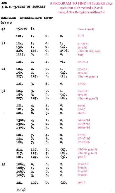
Program 1 demonstrates the operation of all the Atlas instructions implemented in the model. Program 2 is a matrix multiplication program, designed to show in particular the operation of the scalar (dot) product calculation that forms the inner loop of matrix multiplication. Most early supercomputers were designed specifically to perform well on this problem, e.g. especially the Cray 1 of 1976. Program 3 is is an adaptation of a program that finds values for the lengths of the sides of Pythagorean right triangles, i.e. it computes values of a, b, c such that a² + ² = c² and a, b, c < k, where k is a constant set at the start of the program..

The files for version 4 can be downloaded from atlas_v4.1.zip.

Instructions on how to use HASE models can be found at Downloading, Installing and Using HASE.

The HASE user interface window contains three panes. Figure 1 shows an image of this interface with the simulation model of Atlas in the main (right hand) Project View pane, model parameters (e.g. register and store contents) in the (left hand) Project Inspector pane. The lower, Output pane shows information produced by HASE. The icons in the top row allow the user to load a model, compile it, run the simulation code thus created and to load the trace file produced by running a simulation back into the model for animation.

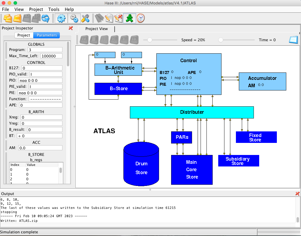
Figure 1. The Atlas simulation model loaded into HASE

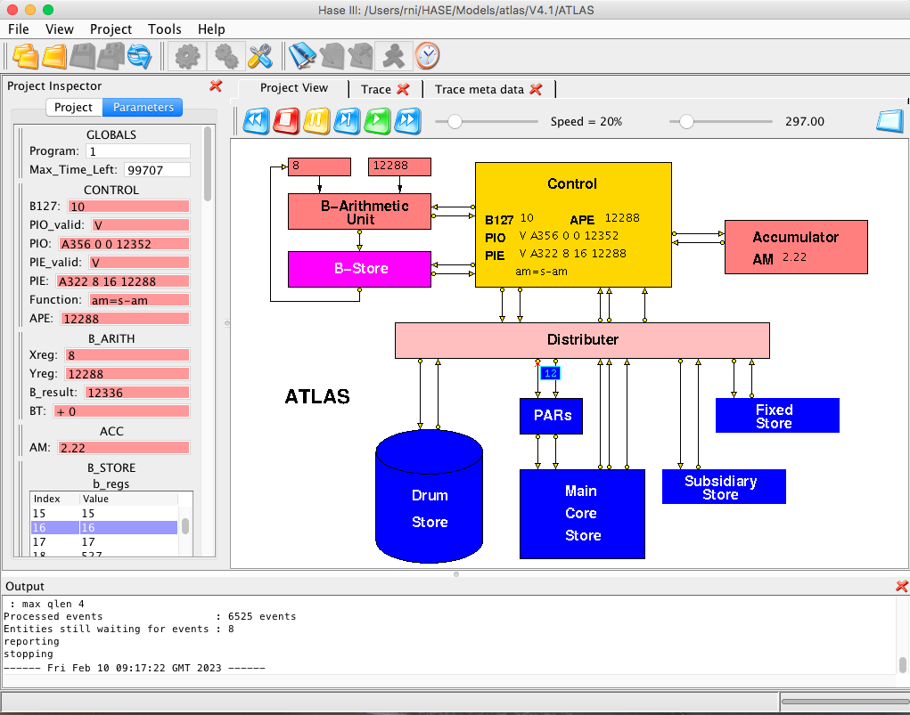
Once a trace file has been loaded, the animation control icons at the top of the Project View window become active (Figure 2). From left to right, these allow the animation to be rewound, stopped, paused, single stepped, run or fast forwarded to the end. As the animation proceeds, packets of information can be seen passing between entities while the entities themselves change colour to reflect their states (idle, busy, waiting).

Figure 2. The Atlas simulation model during animation

The model contains 11 entities: the B-Arithmetic Unit, the B-Store, the Control unit, the Console, the Accumulator, the Distributer, the Page Address Registers (PARs) and the Drum, Core, Subsidiary and Fixed Stores. In Figure 2 the B-Store, the Accumulator and the Distributer are busy, the Control unit is waiting and the rest are idle.

The Atlas instruction set

Atlas had a 48-bit instruction word made up of a 10-bit function code, two 7-bit index addresses (Ba and Bm) and a 24-bit store address (Figure 3). Functions that operated on the Accumulator (A-codes) were thus one-address with double B-modification. B-line 0 always returned a value of 0, thus allowing for singly modified or unmodified accesses. The most significant bit of the address field distinguished between user addresses and system addresses, while the three least significant bits were used to address one of eight 6-bit characters within a store word.

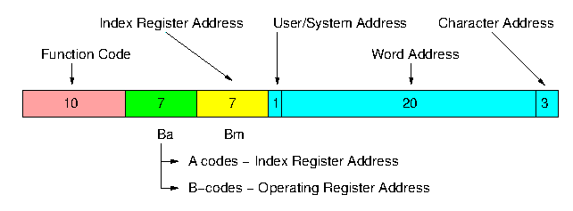
Figure 3. Atlas instruction format

The B-codes involved operations on one of the 128 B-lines specified by the Ba field in the instruction, Bm being used to specify a single modifier. The B-store was implemented as a fast core store (0.7 microsecs cycle time) of 120 24-bit words, together with eight flip-flop registers which served special purposes. These included the floating-point accumulator exponent, for example, and the three control registers (or program counters) used for user programs, extracode and interrupt control. The existence of these three control registers allowed the machine to switch rapidly from one context to another, while their inclusion within the addressable B-store avoided the need for separate control transfer functions. Extracodes were a set of functions which gave access to some 250 built-in subroutines held in the high-speed (0.5 microsecs) read-only fixed store. These included the more complex mathematical functions such as sin, log, etc., peripheral control orders, input/output conversion routines, etc. The extracodes made use of 30 of the B-lines, leaving 90 for use as index registers or fixed-point accumulators in user programs.

User addresses in Atlas (defined by a 0 in their most significant address bit) referred to a 1M word virtual address space, and were translated into real addresses through a set of page registers. The real store consisted of a total of 112K words of core and drum storage, combined together through the paging mechanism so as to appear to the user as a one-level store [1]. Thus a user's total working store requirements could not exceed this amount, but code and data could be placed in any convenient part of the virtual address space. This led to an informal segmentation of the address space, a concept developed formally at MIT in MULTICS and at Manchester in MU5, the successor to Atlas.

Atlas addresses with a 1 in the most significant bit were system addresses rather than user virtual addresses, and referred to the fixed store (containing the extracodes), the subsidiary store (used as working space by the extracodes and operating system), or the V-store. The latter contained the various registers needed to control the tape decks, input/output devices, paging mechanism, etc., thus avoiding the need for special functions for this purpose. This technique of incorporating peripherals into the address space was subsequently used in a number of computer systems, notably the DEC PDP-11, and is now in common use as 'memory-mapped I/O'.

The Simulation Model

In any simulation modelling system there is a trade-off between accuracy and performance. HASE was designed primarily as a high-level visualisation tool for computer architecture students and therefore simulates systems at register/word level rather than bit level. This inevitably imposes some limitations on the way models can be constructed, e.g. registers are modelled using typed variables and stores are modelled as arrays of typed variables. Thus the HASE Atlas simulation model is intended to provide a visual demonstration of the workings of the processor and memory system, rather than being designed to run real Atlas programs.

The Drum and Core Stores

HASE models memories as arrays of elements which can be integers, floating-point numbers or instructions. Since these elements cannot be mixed together in a single array, the model takes advantage of the Atlas paging system by modelling the Drum Store and the Core Store as sets of blocks, with each block made up of 512 words, as in Atlas (though only 256 words are instantiated in the model for performace reasons), but with different blocks containing different types of element.

At the start of each simulation the program and its data are contained in the Drum Store while the Core Store is empty (i.e. contains zeroes). The instructions and operands for the three programs are in Drum Store blocks as shown in the following list:

DRUM STORE Block 0		Program 1 instructions
DRUM STORE Block 1		Program 2 instructions
DRUM STORE Block 2		Program 1 integers
DRUM STORE Block 3		Program 1 reals
DRUM STORE Block 4		Program 3 instructions
DRUM STORE Block 5		Program 2 reals
DRUM STORE Block 6		Program 3 integers

Core Store Block 0 is modelled as an instruction array, Block 1 as an integer array and Block 2 as a real (i.e. floating-point) array. The Fixed Store and Subsidiary Store are also included as entities in the model. The Subsidiary Store is used only in the third of the example programs while the Fixed Store is not used at all.

The Page Address Registers

The PARs are modelled as a set of registers, each of which contains (from left to right in the Project Inspector pane) a use bit, a valid bit and an address. The initiallsation file for the Page Address Registers (PARs) sets all the PARs to zero (and thus invalid) at the start of a simulation. The first action in the simulation of each of the three programs is an instruction access to word 0 of the virtual memory (because B127, the Program Counter, is initially set to 0). This causes a page fault in the PARs. The PARs and the Drum Store are coded to imitate the actions of the Atlas Supervisor (the Atlas operating system). The Hase++ code for d_store.hase encodes the mapping of the Drum Store blocks to the appropriate Core Store blocks and initiates the required transfers (unseen in the simulation) at the behest of the Page Address Registers whenever a page fault occurs, e.g. when the first page fault occurs, the instructions in page 0 of the virtual address space are copied from block 0 of the Drum Store to block 0 of the Core Store and the first PAR is set to point to it. The actual movement of data is not shown in the visualistion (it would be very tedious to watch) but the Core Store contents are shown being updated when the first store request reaches it. Subsequently, when accesses are made for data, similar actions occur on the first access. A full demonstration of the paging system is beyond the scope of the current model.

Instruction Format

Instructions are modelled as closely as possible to the Atlas format, with the Ba, Bm and Address fields being modelled as integers. However, HASE models the function field of instructions as elements of an enumerated type and these elements cannot be integers. Functions in the model are therefore of the form A314, B121, etc, which actually aids legibility. The model also includes four Extracodes, detailed below.

Floating-point Arithmetic

The model implements floating-point arithmetic using the floating-point operations provided by the underlying hardware of the computer on which the simulation runs, accessed via standard C++ operations. This is not an accurate representation of the way Atlas performed these operations, of course, but is adequate for the purposes of this demonstration. To simulate the 48-bit floating-point arithmetic used in Atlas would require bit-level coding of the Accumulator unit and would not be especially instructive, except to floating-point arithmetic enthusiasts.

For the same reasons, the model does not implement the full set of Atlas floating-point instructions, nor does it attempt to model the Accumulator as a double-length register. It just implements simple load, store, add, subtract, multiply and divide operations on AM, the most significant half of the Atlas double-length accumulator. Also, B124, the floating-point exponent register in Atlas, is not implemented.

Instruction Test Program (Program 1)

Program 1 in the model is shown in Table 1. Its instructions are in Page 0 of the virtual address space, initially held in Block 0 of the Drum Store and copied into Block 0 of the Core Store following the page fault caused by the first instruction access. It uses some of the integers in virtual page 1, held in Block 2 of the Drum Store and copied into Block 1 of the Core Store when the first integer operand access causes a page fault, and likewise the floating-point numbers in virtual page 2, initially held in Block 3 of the Drum Store and copied into Block 2 of the Core Store. The program executes each of the instructions implemented in the model. As well as the A and B functions, the model uses an Extracode, E1121. E1121 is a feature of the model rather than Atlas itself. It writes to B120 and this causes B registers 1-119 to be loaded with values 1-119 respectively, some of which are used by the program. Table 1 shows the actions performed for each instruction and the resulting outcome.

AM = Accumulator, VS = Virtual Store, CS B2W8 = Core Store Block 2, Word 8

B127	Instruction	Action	Result
0	E1121 0 0 0	Loads B1-119	B1-119 = 1-119
1	B121 0 0 42	Tries to load B0 with 42	B0 = 0
2	B101 18 0 8312	Loads B18 from VS word 1039 (for use later)	B18 = 527
3	A315 0 0 12296	Loads AM with VS word 1537 & negates AM	AM = -2.2
4	A314 0 0 12288	Loads AM from VS word 1536	AM = 1.1
5	A363 0 16 12288	Multiplies AM by VS word 1538 & negates AM	AM = -3.63
6	A320 24 40 12288	Adds VS word 1544 to AM	AM = 6.2
7	A362 24 32 12288	Multiplies AM by VS word 1543	AM = 54.56
8	A374 8 24 12288	Divides AM by VS word 1540	AM = 9.92
9	A321 8 40 12288	Subtracts VS word 1542 from AM	AM = 2.22
10	A322 8 16 12288	Subtracts AM from VS word 1539	AM = 2.18
11	A356 0 0 12352	Stores AM in VS word 1544	CS B2W8 = 2.18
12	A346 0 0 12360	Stores AM in VS word 1545 and sets AM = 0	CS B2W9 = 2.18, AM = 0
13	B100 11 0 8192	Subtracts value in B11 from VS word 1024 (= 512)	B11 = 501
14	B101 12 0 8200	Loads VS word 1025 to B12	B12 = 513
15	B102 13 0 8208	Subtracts VS word 1026 from B13	B13 = -501
16	B103 14 0 8216	Loads negated value in VS word 1027 to B14	B14 = -515
17	B104 15 0 8216	Adds VS word 1028 to B15	B15 = 531
18	B104 16 32 8224	Adds VS word (1037+4) to B16	B16 = 545
19	B106 17 0 8296	Forms XOR of VS word 1031 with B17	B17 = 534
20	B107 18 0 8240	Forms AND of VS word 1030 with B18	B18 = 523
21	B147 19 0 8216	Forms OR of VS word 1027 with B19	B19 = 531
22	B110 21 0 8256	Subtracts B21 from VS word 1032	CS B1W8 = 499
23	B111 21 0 8264	Stores negated value in B21 in VS word 1033	CS B1W9 = -21
24	B112 21 0 8272	Subtracts VS word 1034 from B21	CS B1W10 = -501
25	B113 23 0 8288	Stores B23 in VS word 1035	CS B1W11 = 23
26	B114 24 0 8288	Adds B24 to VS word 1036	CS B1W12 = 548
27	B116 26 0 8296	Forms XOR of B26 with VS word 1037	CS B1W13 = 535
28	B117 22 24 8280	Forms AND of VS word (1035+3) with B22	CS B1W14 = 6
29	B120 27 0 345	Subtracts value in B27 from 345	B27 = 318
30	B121 28 127 77654	Loads B28 with 77654 + value in B127	B28 = 77682
31	B122 29 0 54321	Subtracts 54321 from B29	B29 = -54292
32	B123 30 0 -8965	Loads -(-8965) to B30	B30 = 8965
33	B124 31 31 0	Adds B31 to itself	B31 = 62
34	B126 32 0 21	Forms XOR of B32 with 21	B32 = 53
35	B167 33 7 99	Forms OR of B33 with 99 + B7	B33 = 107
36	B164 34 33 35	Adds B33 & 35 to B34	B34 = 69
37	B165 35 33 62	Loads B35 with B33 & 62	B35 = 42
38	B101 36 0 1024	Loads B36 with CS word 512	B36 = 512
39	B163 36 0 52	Circular shift right B36 1 place and subtract 52	B36 = 204
40	B121 37 0 0	Sets B37 to 0	B37 = 0
41	B125 37 0 7	Circular shift B37 left 6 places and add 7	B37 = 7
42	B125 37 0 8	Circular shift B37 left 6 places and add 8	B37 = 456
43	B125 37 0 3	Circular shift B37 left 6 places and add 3	B37 = 29187
44	B125 37 0 5	Circular shift B37 left 6 places and add 5	B37 = 1867973
45	B125 37 0 0	Circular shift B37 left 6 places and add 0	B37 = 2109767
46	B127 37 0 63	Forms AND of B37 with 63 (selects 1^st value added)	B37 = 7
47	B150 38 0 8320	Sets BT according to VS word 1040 - B38	bt = +, /0
48	B152 38 0 8320	Sets BT according to B38 - VS word 1040	bt = -. /0
49	B170 38 0 38	Sets BT according to B38 - 38	bt = +, 0
50	B172 38 0 29	Sets BT according to B38 - 39	bt = -, /0
51	B200 40 39 540	If B39 /=0, add 1 to B39, B40 = 540	B39 = 40, B40 = 540
52	B201 42 41 541	If B41 /=0, add 2 to B41, B42 = 541	B41 = 43, B42 = 541
53	B202 44 43 542	If B43/=0, add -1 to B43, B44 = 542	B43 = 42, B44 = 542
54	B203 46 45 543	If B45 /=0, add -2 to B45, B46 = 543	B45 = 43, B46 = 543
55	B200 46 0 544	If B0 /=0, add 1 to B0, B46 = 544 - test fails	B0 = 0, B46 = 543
56	B220 48 47 544	If bt /=0, add 1 to B47, B48 = 544	B47 = 48, B48 = 544
57	B221 50 49 545	If bt /=0, add 2 to B49, B50 = 545	B49 = 51, B50 = 545
58	B222 52 51 546	If bt /=0, add -1 to B51, B52 = 546	B51 = 50, B52 = 546
59	B223 55 53 547	If bt /=0, add -2 to B53, B55 = 547	B53 = 51, B54 = 547
60	B121 56 0 65	Loads B56 with 65	B56 = 65
61	B210 57 56 111	If B56 odd, load B57 with 111	B57 = 111
62	B121 56 0 64	Loads B56 with 64	B56 = 64
63	B211 58 56 222	If B56 even, load B58 with 222	B58 = 222
64	B121 56 0 0	Loads B56 with 0	B56 = 0
65	B214 59 56 333	If B56 = 0, load B59 with 333	B59 = 333
66	B121 56 0 42	Loads B56 with 42	B56 = 42
67	B215 60 56 444	If B56 /= 0, load B60 with 444	B60 = 444
68	B216 61 56 555	If B56 >=0, load B61 with 555	B61 = 555
69	B217 62 56 666	If B56 < 0, load B62 with 666 - test fails	B62 = 62
70	B121 56 0 -89	Loads B56 with -89	B56 = -89
71	B217 63 56 777	If B56 < 0, load B63 with 777	B63 = 777
72	B217 127 56 82	If B56 < 0, absolute jump to 82	B127 = 82
73	B172 64 0 64	Sets BT according to B64 - 64	bt = +, 0
74	B224 65 0 1111	If bt =0, B65 = 1111	B65 = 1111
75	B172 64 0 63	Sets BT according to B64 - 63	bt = +, /0
76	B225 66 0 2222	If bt /=0, B66 = 2222	B66 = 2222
77	B226 67 0 3333	If bt >=0, B67 = 3333	B67 = 3333
78	B172 64 0 65	Sets BT according to B64 - 65	bt = -, /0
79	B227 68 0 4444	If bt <0, B68 = 4444	B68 = 4444
80	B226 68 0 5555	If bt >=0, B68 = 5555 - test fails	B68 = 4444
81	STOP	Stops the simulation
82	B210 127 68 61	If B68 odd, B127 = 61 - test fails	B127 = 61
83	B122 127 0 10	Relative jump back to 73	B127 = 73

Table 1. The Instruction Test Program

Matrix Multiplication Program (Program 2)

The matrix multiplication program multiplies together a 4x3 matrix X and a 3x4 matrix Y to produce a 4x4 matrix Z, as shown in Figure 4. The first element of the first row of Z is the scalar (dot) product of the first row of X and the first column of Y, the second is the scalar product of the first row of X with the second column of Y, etc.

Table 2 shows the program, which is in the form of a triple nested loop. The outer loop increments the X row at each iteration, the middle loop increments the Y column at each iteration while the inner loop forms the scalar products.

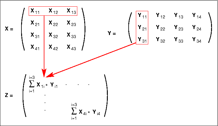
Figure 4. Matrix multiplication example

B127	Instruction	Purpose/Action	Result
0	B121 1 24 0	B1 = X row length / Y column length (x8)	B1 = 24
1	B121 2 32 0	B2 = X column length / Y row length (x8)	B2 = 32
2	B121 3 0 0	B3 = current X row number	B3 = 0
3	B121 4 0 0	B4 = address of first column of current X row	B4 = 0
4	B121 5 0 0	B5 = current X column number	B5 = 0
5	B121 6 0 0	B6 = current Y column number	B6 = 0
6	B121 7 0 0	B7 = address of Y row element	B7 = 0
7	B121 8 0 0	B8 = Z index number (x8)	B8 = 0
8	A314 4 5 12288	Start of Loop: Loads ACC with element of X	ACC = X_ji
9	A362 6 7 12384	Multiplies ACC by element of Y	ACC * Y_ij
10	A320 8 0 12480	Adds element of Z to ACC
11	A356 8 0 12480	Writes ACC to element of Z
12	B124 5 0 8	Increment word address of X column number	B5 + 8
13	B124 7 2 0	Increment word address of Y row number	B7 + B2
14	B172 5 1 0	Test B5 against B1	Sets BT
15	B225 127 0 8	If BT /=0, jump back to start of Loop	B127 = 8
16	B121 5 0 0	Resets X column number to 0	B5 = 0
17	B124 6 0 8	Increments Y column number	B6 + 8
18	B121 7 0 0	Resets Y row number to 0	B7 = 0
19	B124 8 0 8	Increments Z index	B8 + 8
20	B172 6 2 0	Test B6 against B1	Sets BT
21	B225 127 0 8	If BT /=0, jump back to start of Loop	B127 = 8
22	B124 3 0 8	Increments X row number	B3 + 8
23	B124 4 1 0	Increment X row address	B4 + B1
24	B121 6 0 0	Resets Y column number	B6 = 0
25	B172 3 2 0	Tests B3 against B2	Sets BT
26	B225 127 0 8	If BT /=0, jump back to start of Loop	B127 = 8
27	STOP

Table 2. The matrix multiplication program

Sums of Squares (Program 3)

Program 3 is a version of a program written by John Buckle in 1962 as a Ferranti training exercise. Figure 5 shows the original code with comments (which include one minor mistake) and the corresponding HASE Atlas simulation code. The value of k is in virtual store word 1024. The program uses three extracodes E1302, E1064 and E1067. E1302 is a B multiply instruction, implemented in the model simply as an instruction executed directly in the B Arithmetic unit. E1064 and E1067 are implemented by the Control Unit and write values into the Subsidiary Store which are printed at the end of the simulation run in the output pane of the HASE GUI. This is not how it would have worked in the real Atlas, of course, but simply a device to enable the sum of squares program to be demonstrated at the Atlas 50^th Anniversary Symposium.

The value of k in the model is set at 15, so the model produces the results:

3, 4, 5
5, 12, 13
6, 8, 10
9, 12, 15

B127
0		B121 8 0 0
1		B121 1 0 0
2	1)	B124 1 0 1
3		B150 1 0 8192
4		B226 127 0 6 if bt>=0, skip next
5		STOP
6		B121 2 1 -1 b2=b1-1
7	2)	B124 2 0 1 b2=b2+1
8		B150 2 0 8192 bt=k-b2
9		B227 127 0 2 if bt>=o, ->1)
10		B121 3 2 0 b3 = b2
11	3)	B124 3 0 1 b3=b3+1
12		B150 3 0 8192 bt=k-b3
13		B227 127 0 7 if bt>=0, ->2)
14		B121 4 1 0 b4=b1
15		B121 5 2 0 b5=b2
16		B121 6 3 0 b6=b3
17		E1302 4 1 0 b4=b4*b1
18		E1302 5 2 0 b5=b5*b2
19		B1302 6 3 0 b6=b6*b3
20		B121 7 4 0 b7=b4
21		B124 7 5 0 b7=b7+b5
22		B122 7 6 0 b7=b7-b6
23		B214 127 7 26 if b7=0, ->5)
24		B217 127 7 7 if b7<0, ->2)
25		B121 127 0 11 -> 3)
26	5)	E1064 0 0 0 print NL
27		E1067 1 0 0 print b1
27		E1067 2 0 0 print b2
27		E1067 3 0 0 print b3
29		B124 8 0 24 b8=b8+24
30		B121 127 0 7 -> 2)

Figure 5. Sums of Squares

Reference

^ T. Kilburn, D.B.G. Edwards, M.J. Lanigan and F.H. Sumner
"One-level Storage System"
IRE Trans., Vol EC-11, pp 223-234 1962

Return to Computer Architecture Simulation Models

HASE Project
Institute for Computing Systems Architecture, School of Informatics, University of Edinburgh
Last change 8/02/2023